Problem: Only about 11% of customers at a Portuguese bank purchased long term deposits (between 2008 and 2013). How can the bank increase these numbers?
This is a telemarketing campaign, so time is money! Therefore, what we want to maximize is the number of sales (during a fixed time period, eg. 40 hours), and I propose that targeting customers based only on their occupation will improve overall sales. Thus the key performance indicator (KPI) that we want to optimize is the time needed to ensure that at least one sale occurs.
Exploratory Data Analysis
As you probably know, data scientists spend the majority of their time in cleaning up data. I converted a few variables into binary variables, converted some strings (day) to integers, and the same with month. After cleaning up the data we can summarize the data on a high level. In this case, our typical customer is 40 years old, married, works in the admin field, graduated from university and is contacted via a cell phone.
Stats on the current campaign:
- Primarily conducted during the summer months, particularly April
- Calls were made nearly uniform during the week (day)
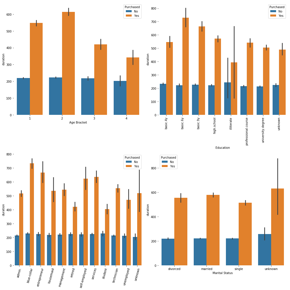
- Calls that resulted in no purchase lasted an average of 3.7 minutes and those that did result in a sale lasted an average of 9.2 minutes
- Each customer was contacted an average of 2.5 times during this campaign
Stats on previous campaign(s):
- After being contacted (for a previous campaign), an average of 962 days passed
- During the last campaign, 1 in every 5.8 customers were contacted at least once
- Every customer was contacted at least once during the current campaign
- 24.4% of customers purchased a long-term deposit during the previous campaign
- 86.3% of all customers were not contacted at all during the previous campaign
- Which means only 13.6% of all customers were contacted at least once during both campaigns
The standard deviation of the social-economic variables are high (relative to it’s mean).
Automated Profiling
Gathering descriptive statistics can be a tedious process. Gladly, there are libraries that exist that perform all of the data crunching for you. They output a very clear profile of your data. pandas-profiling is one of them. That library offers out-of-the-box statistical profiling of your dataset. Since the dataset we are using is tidy and standardized, we can use the library right away on our dataset.
Dataset info
| Number of variables |
22 |
| Number of observations |
41188 |
| Total Missing (%) |
3.9% |
| Total size in memory |
5.5 MiB |
| Average record size in memory |
141.0 B |
Variables types
| Numeric |
11 |
| Categorical |
5 |
| Boolean |
4 |
| Date |
0 |
| Text (Unique) |
0 |
| Rejected |
2 |
| Unsupported |
0 |
| Distinct count |
78 |
| Unique (%) |
0.2% |
| Missing (%) |
0.0% |
| Missing (n) |
0 |
| Infinite (%) |
0.0% |
| Infinite (n) |
0 |
| Mean |
40.024 |
| Minimum |
17 |
| Maximum |
98 |
| Zeros (%) |
0.0% |
Quantile statistics
| Minimum |
17 |
| 5-th percentile |
26 |
| Q1 |
32 |
| Median |
38 |
| Q3 |
47 |
| 95-th percentile |
58 |
| Maximum |
98 |
| Range |
81 |
| Interquartile range |
15 |
Descriptive statistics
| Standard deviation |
10.421 |
| Coef of variation |
0.26037 |
| Kurtosis |
0.79131 |
| Mean |
40.024 |
| MAD |
8.4615 |
| Skewness |
0.7847 |
| Sum |
1648511 |
| Variance |
108.6 |
| Memory size |
321.9 KiB |
| Value |
Count |
Frequency (%) |
|
| 31 |
1947 |
4.7% |
|
| 32 |
1846 |
4.5% |
|
| 33 |
1833 |
4.5% |
|
| 36 |
1780 |
4.3% |
|
| 35 |
1759 |
4.3% |
|
| 34 |
1745 |
4.2% |
|
| 30 |
1714 |
4.2% |
|
| 37 |
1475 |
3.6% |
|
| 29 |
1453 |
3.5% |
|
| 39 |
1432 |
3.5% |
|
| Other values (68) |
24204 |
58.8% |
|
Minimum 5 values
| Value |
Count |
Frequency (%) |
|
| 17 |
5 |
0.0% |
|
| 18 |
28 |
0.1% |
|
| 19 |
42 |
0.1% |
|
| 20 |
65 |
0.2% |
|
| 21 |
102 |
0.2% |
|
Maximum 5 values
| Value |
Count |
Frequency (%) |
|
| 91 |
2 |
0.0% |
|
| 92 |
4 |
0.0% |
|
| 94 |
1 |
0.0% |
|
| 95 |
1 |
0.0% |
|
| 98 |
2 |
0.0% |
|
| Distinct count |
4 |
| Unique (%) |
0.0% |
| Missing (%) |
0.0% |
| Missing (n) |
0 |
| Distinct count |
42 |
| Unique (%) |
0.1% |
| Missing (%) |
0.0% |
| Missing (n) |
0 |
| Infinite (%) |
0.0% |
| Infinite (n) |
0 |
| Mean |
2.5676 |
| Minimum |
1 |
| Maximum |
56 |
| Zeros (%) |
0.0% |
Quantile statistics
| Minimum |
1 |
| 5-th percentile |
1 |
| Q1 |
1 |
| Median |
2 |
| Q3 |
3 |
| 95-th percentile |
7 |
| Maximum |
56 |
| Range |
55 |
| Interquartile range |
2 |
Descriptive statistics
| Standard deviation |
2.77 |
| Coef of variation |
1.0788 |
| Kurtosis |
36.98 |
| Mean |
2.5676 |
| MAD |
1.6342 |
| Skewness |
4.7625 |
| Sum |
105754 |
| Variance |
7.673 |
| Memory size |
321.9 KiB |
| Value |
Count |
Frequency (%) |
|
| 1 |
17642 |
42.8% |
|
| 2 |
10570 |
25.7% |
|
| 3 |
5341 |
13.0% |
|
| 4 |
2651 |
6.4% |
|
| 5 |
1599 |
3.9% |
|
| 6 |
979 |
2.4% |
|
| 7 |
629 |
1.5% |
|
| 8 |
400 |
1.0% |
|
| 9 |
283 |
0.7% |
|
| 10 |
225 |
0.5% |
|
| Other values (32) |
869 |
2.1% |
|
Minimum 5 values
| Value |
Count |
Frequency (%) |
|
| 1 |
17642 |
42.8% |
|
| 2 |
10570 |
25.7% |
|
| 3 |
5341 |
13.0% |
|
| 4 |
2651 |
6.4% |
|
| 5 |
1599 |
3.9% |
|
Maximum 5 values
| Value |
Count |
Frequency (%) |
|
| 40 |
2 |
0.0% |
|
| 41 |
1 |
0.0% |
|
| 42 |
2 |
0.0% |
|
| 43 |
2 |
0.0% |
|
| 56 |
1 |
0.0% |
|
| Distinct count |
26 |
| Unique (%) |
0.1% |
| Missing (%) |
0.0% |
| Missing (n) |
0 |
| Infinite (%) |
0.0% |
| Infinite (n) |
0 |
| Mean |
-40.503 |
| Minimum |
-50.8 |
| Maximum |
-26.9 |
| Zeros (%) |
0.0% |
Quantile statistics
| Minimum |
-50.8 |
| 5-th percentile |
-47.1 |
| Q1 |
-42.7 |
| Median |
-41.8 |
| Q3 |
-36.4 |
| 95-th percentile |
-33.6 |
| Maximum |
-26.9 |
| Range |
23.9 |
| Interquartile range |
6.3 |
Descriptive statistics
| Standard deviation |
4.6282 |
| Coef of variation |
-0.11427 |
| Kurtosis |
-0.35856 |
| Mean |
-40.503 |
| MAD |
3.9383 |
| Skewness |
0.30318 |
| Sum |
-1668200 |
| Variance |
21.42 |
| Memory size |
321.9 KiB |
| Value |
Count |
Frequency (%) |
|
| -36.4 |
7763 |
18.8% |
|
| -42.7 |
6685 |
16.2% |
|
| -46.2 |
5794 |
14.1% |
|
| -36.1 |
5175 |
12.6% |
|
| -41.8 |
4374 |
10.6% |
|
| -42.0 |
3616 |
8.8% |
|
| -47.1 |
2458 |
6.0% |
|
| -31.4 |
770 |
1.9% |
|
| -40.8 |
715 |
1.7% |
|
| -26.9 |
447 |
1.1% |
|
| Other values (16) |
3391 |
8.2% |
|
Minimum 5 values
| Value |
Count |
Frequency (%) |
|
| -50.8 |
128 |
0.3% |
|
| -50.0 |
282 |
0.7% |
|
| -49.5 |
204 |
0.5% |
|
| -47.1 |
2458 |
6.0% |
|
| -46.2 |
5794 |
14.1% |
|
Maximum 5 values
| Value |
Count |
Frequency (%) |
|
| -33.0 |
172 |
0.4% |
|
| -31.4 |
770 |
1.9% |
|
| -30.1 |
357 |
0.9% |
|
| -29.8 |
267 |
0.6% |
|
| -26.9 |
447 |
1.1% |
|
| Distinct count |
26 |
| Unique (%) |
0.1% |
| Missing (%) |
0.0% |
| Missing (n) |
0 |
| Infinite (%) |
0.0% |
| Infinite (n) |
0 |
| Mean |
93.576 |
| Minimum |
92.201 |
| Maximum |
94.767 |
| Zeros (%) |
0.0% |

Quantile statistics
| Minimum |
92.201 |
| 5-th percentile |
92.713 |
| Q1 |
93.075 |
| Median |
93.749 |
| Q3 |
93.994 |
| 95-th percentile |
94.465 |
| Maximum |
94.767 |
| Range |
2.566 |
| Interquartile range |
0.919 |
Descriptive statistics
| Standard deviation |
0.57884 |
| Coef of variation |
0.0061858 |
| Kurtosis |
-0.82981 |
| Mean |
93.576 |
| MAD |
0.50981 |
| Skewness |
-0.23089 |
| Sum |
3854200 |
| Variance |
0.33506 |
| Memory size |
321.9 KiB |
| Value |
Count |
Frequency (%) |
|
| 93.994 |
7763 |
18.8% |
|
| 93.91799999999999 |
6685 |
16.2% |
|
| 92.89299999999999 |
5794 |
14.1% |
|
| 93.444 |
5175 |
12.6% |
|
| 94.465 |
4374 |
10.6% |
|
| 93.2 |
3616 |
8.8% |
|
| 93.075 |
2458 |
6.0% |
|
| 92.20100000000001 |
770 |
1.9% |
|
| 92.963 |
715 |
1.7% |
|
| 92.431 |
447 |
1.1% |
|
| Other values (16) |
3391 |
8.2% |
|
Minimum 5 values
| Value |
Count |
Frequency (%) |
|
| 92.20100000000001 |
770 |
1.9% |
|
| 92.37899999999999 |
267 |
0.6% |
|
| 92.431 |
447 |
1.1% |
|
| 92.469 |
178 |
0.4% |
|
| 92.649 |
357 |
0.9% |
|
Maximum 5 values
| Value |
Count |
Frequency (%) |
|
| 94.199 |
303 |
0.7% |
|
| 94.215 |
311 |
0.8% |
|
| 94.465 |
4374 |
10.6% |
|
| 94.601 |
204 |
0.5% |
|
| 94.76700000000001 |
128 |
0.3% |
|
| Distinct count |
2 |
| Unique (%) |
0.0% |
| Missing (%) |
0.0% |
| Missing (n) |
0 |
| cellular |
26144
|
| telephone |
15044
|
| Distinct count |
5 |
| Unique (%) |
0.0% |
| Missing (%) |
0.0% |
| Missing (n) |
0 |
| Infinite (%) |
0.0% |
| Infinite (n) |
0 |
| Mean |
1.9796 |
| Minimum |
0 |
| Maximum |
4 |
| Zeros (%) |
20.7% |
Quantile statistics
| Minimum |
0 |
| 5-th percentile |
0 |
| Q1 |
1 |
| Median |
2 |
| Q3 |
3 |
| 95-th percentile |
4 |
| Maximum |
4 |
| Range |
4 |
| Interquartile range |
2 |
Descriptive statistics
| Standard deviation |
1.4115 |
| Coef of variation |
0.71304 |
| Kurtosis |
-1.2998 |
| Mean |
1.9796 |
| MAD |
1.2032 |
| Skewness |
0.00055242 |
| Sum |
81535 |
| Variance |
1.9924 |
| Memory size |
321.9 KiB |
| Value |
Count |
Frequency (%) |
|
| 3 |
8623 |
20.9% |
|
| 0 |
8514 |
20.7% |
|
| 2 |
8134 |
19.7% |
|
| 1 |
8090 |
19.6% |
|
| 4 |
7827 |
19.0% |
|
Minimum 5 values
| Value |
Count |
Frequency (%) |
|
| 0 |
8514 |
20.7% |
|
| 1 |
8090 |
19.6% |
|
| 2 |
8134 |
19.7% |
|
| 3 |
8623 |
20.9% |
|
| 4 |
7827 |
19.0% |
|
Maximum 5 values
| Value |
Count |
Frequency (%) |
|
| 0 |
8514 |
20.7% |
|
| 1 |
8090 |
19.6% |
|
| 2 |
8134 |
19.7% |
|
| 3 |
8623 |
20.9% |
|
| 4 |
7827 |
19.0% |
|
| Distinct count |
2 |
| Unique (%) |
0.0% |
| Missing (%) |
0.0% |
| Missing (n) |
0 |
| Distinct count |
1544 |
| Unique (%) |
3.7% |
| Missing (%) |
0.0% |
| Missing (n) |
0 |
| Infinite (%) |
0.0% |
| Infinite (n) |
0 |
| Mean |
258.29 |
| Minimum |
0 |
| Maximum |
4918 |
| Zeros (%) |
0.0% |
Quantile statistics
| Minimum |
0 |
| 5-th percentile |
36 |
| Q1 |
102 |
| Median |
180 |
| Q3 |
319 |
| 95-th percentile |
752.65 |
| Maximum |
4918 |
| Range |
4918 |
| Interquartile range |
217 |
Descriptive statistics
| Standard deviation |
259.28 |
| Coef of variation |
1.0038 |
| Kurtosis |
20.248 |
| Mean |
258.29 |
| MAD |
171.67 |
| Skewness |
3.2631 |
| Sum |
10638243 |
| Variance |
67226 |
| Memory size |
321.9 KiB |
| Value |
Count |
Frequency (%) |
|
| 85 |
170 |
0.4% |
|
| 90 |
170 |
0.4% |
|
| 136 |
168 |
0.4% |
|
| 73 |
167 |
0.4% |
|
| 124 |
164 |
0.4% |
|
| 87 |
162 |
0.4% |
|
| 72 |
161 |
0.4% |
|
| 104 |
161 |
0.4% |
|
| 111 |
160 |
0.4% |
|
| 106 |
159 |
0.4% |
|
| Other values (1534) |
39546 |
96.0% |
|
Minimum 5 values
| Value |
Count |
Frequency (%) |
|
| 0 |
4 |
0.0% |
|
| 1 |
3 |
0.0% |
|
| 2 |
1 |
0.0% |
|
| 3 |
3 |
0.0% |
|
| 4 |
12 |
0.0% |
|
Maximum 5 values
| Value |
Count |
Frequency (%) |
|
| 3631 |
1 |
0.0% |
|
| 3643 |
1 |
0.0% |
|
| 3785 |
1 |
0.0% |
|
| 4199 |
1 |
0.0% |
|
| 4918 |
1 |
0.0% |
|
| Distinct count |
8 |
| Unique (%) |
0.0% |
| Missing (%) |
0.0% |
| Missing (n) |
0 |
| university.degree |
12168
|
| high.school |
9515
|
| basic.9y |
6045
|
| Other values (5) |
13460
|
| Distinct count |
10 |
| Unique (%) |
0.0% |
| Missing (%) |
0.0% |
| Missing (n) |
0 |
| Infinite (%) |
0.0% |
| Infinite (n) |
0 |
| Mean |
0.081886 |
| Minimum |
-3.4 |
| Maximum |
1.4 |
| Zeros (%) |
0.0% |
Quantile statistics
| Minimum |
-3.4 |
| 5-th percentile |
-2.9 |
| Q1 |
-1.8 |
| Median |
1.1 |
| Q3 |
1.4 |
| 95-th percentile |
1.4 |
| Maximum |
1.4 |
| Range |
4.8 |
| Interquartile range |
3.2 |
Descriptive statistics
| Standard deviation |
1.571 |
| Coef of variation |
19.185 |
| Kurtosis |
-1.0626 |
| Mean |
0.081886 |
| MAD |
1.4228 |
| Skewness |
-0.7241 |
| Sum |
3372.7 |
| Variance |
2.4679 |
| Memory size |
321.9 KiB |
| Value |
Count |
Frequency (%) |
|
| 1.4 |
16234 |
39.4% |
|
| -1.8 |
9184 |
22.3% |
|
| 1.1 |
7763 |
18.8% |
|
| -0.1 |
3683 |
8.9% |
|
| -2.9 |
1663 |
4.0% |
|
| -3.4 |
1071 |
2.6% |
|
| -1.7 |
773 |
1.9% |
|
| -1.1 |
635 |
1.5% |
|
| -3.0 |
172 |
0.4% |
|
| -0.2 |
10 |
0.0% |
|
Minimum 5 values
| Value |
Count |
Frequency (%) |
|
| -3.4 |
1071 |
2.6% |
|
| -3.0 |
172 |
0.4% |
|
| -2.9 |
1663 |
4.0% |
|
| -1.8 |
9184 |
22.3% |
|
| -1.7 |
773 |
1.9% |
|
Maximum 5 values
| Value |
Count |
Frequency (%) |
|
| -1.1 |
635 |
1.5% |
|
| -0.2 |
10 |
0.0% |
|
| -0.1 |
3683 |
8.9% |
|
| 1.1 |
7763 |
18.8% |
|
| 1.4 |
16234 |
39.4% |
|
euribor3m
Highly correlated
This variable is highly correlated with emp.var.rate and should be ignored for analysis
| Distinct count |
2 |
| Unique (%) |
0.0% |
| Missing (%) |
0.0% |
| Missing (n) |
0 |
| Distinct count |
12 |
| Unique (%) |
0.0% |
| Missing (%) |
0.0% |
| Missing (n) |
0 |
| admin. |
10422
|
| blue-collar |
9254
|
| technician |
6743
|
| Other values (9) |
14769
|
| Distinct count |
2 |
| Unique (%) |
0.0% |
| Missing (%) |
0.0% |
| Missing (n) |
0 |
| Distinct count |
4 |
| Unique (%) |
0.0% |
| Missing (%) |
0.0% |
| Missing (n) |
0 |
| married |
24928
|
| single |
11568
|
| divorced |
4612
|
| Distinct count |
10 |
| Unique (%) |
0.0% |
| Missing (%) |
0.0% |
| Missing (n) |
0 |
| Infinite (%) |
0.0% |
| Infinite (n) |
0 |
| Mean |
5.6079 |
| Minimum |
2 |
| Maximum |
11 |
| Zeros (%) |
0.0% |
Quantile statistics
| Minimum |
2 |
| 5-th percentile |
3 |
| Q1 |
4 |
| Median |
5 |
| Q3 |
7 |
| 95-th percentile |
10 |
| Maximum |
11 |
| Range |
9 |
| Interquartile range |
3 |
Descriptive statistics
| Standard deviation |
2.041 |
| Coef of variation |
0.36395 |
| Kurtosis |
-0.027876 |
| Mean |
5.6079 |
| MAD |
1.661 |
| Skewness |
0.85151 |
| Sum |
230978 |
| Variance |
4.1657 |
| Memory size |
321.9 KiB |
| Value |
Count |
Frequency (%) |
|
| 4 |
13769 |
33.4% |
|
| 6 |
7174 |
17.4% |
|
| 7 |
6178 |
15.0% |
|
| 5 |
5318 |
12.9% |
|
| 10 |
4101 |
10.0% |
|
| 3 |
2632 |
6.4% |
|
| 9 |
718 |
1.7% |
|
| 8 |
570 |
1.4% |
|
| 2 |
546 |
1.3% |
|
| 11 |
182 |
0.4% |
|
Minimum 5 values
| Value |
Count |
Frequency (%) |
|
| 2 |
546 |
1.3% |
|
| 3 |
2632 |
6.4% |
|
| 4 |
13769 |
33.4% |
|
| 5 |
5318 |
12.9% |
|
| 6 |
7174 |
17.4% |
|
Maximum 5 values
| Value |
Count |
Frequency (%) |
|
| 7 |
6178 |
15.0% |
|
| 8 |
570 |
1.4% |
|
| 9 |
718 |
1.7% |
|
| 10 |
4101 |
10.0% |
|
| 11 |
182 |
0.4% |
|
nr.employed
Highly correlated
This variable is highly correlated with euribor3m and should be ignored for analysis
| Distinct count |
27 |
| Unique (%) |
0.1% |
| Missing (%) |
0.0% |
| Missing (n) |
0 |
| Infinite (%) |
0.0% |
| Infinite (n) |
0 |
| Mean |
962.48 |
| Minimum |
0 |
| Maximum |
999 |
| Zeros (%) |
0.0% |
Quantile statistics
| Minimum |
0 |
| 5-th percentile |
999 |
| Q1 |
999 |
| Median |
999 |
| Q3 |
999 |
| 95-th percentile |
999 |
| Maximum |
999 |
| Range |
999 |
| Interquartile range |
0 |
Descriptive statistics
| Standard deviation |
186.91 |
| Coef of variation |
0.1942 |
| Kurtosis |
22.229 |
| Mean |
962.48 |
| MAD |
70.362 |
| Skewness |
-4.9222 |
| Sum |
39642439 |
| Variance |
34936 |
| Memory size |
321.9 KiB |
| Value |
Count |
Frequency (%) |
|
| 999 |
39673 |
96.3% |
|
| 3 |
439 |
1.1% |
|
| 6 |
412 |
1.0% |
|
| 4 |
118 |
0.3% |
|
| 9 |
64 |
0.2% |
|
| 2 |
61 |
0.1% |
|
| 7 |
60 |
0.1% |
|
| 12 |
58 |
0.1% |
|
| 10 |
52 |
0.1% |
|
| 5 |
46 |
0.1% |
|
| Other values (17) |
205 |
0.5% |
|
Minimum 5 values
| Value |
Count |
Frequency (%) |
|
| 0 |
15 |
0.0% |
|
| 1 |
26 |
0.1% |
|
| 2 |
61 |
0.1% |
|
| 3 |
439 |
1.1% |
|
| 4 |
118 |
0.3% |
|
Maximum 5 values
| Value |
Count |
Frequency (%) |
|
| 22 |
3 |
0.0% |
|
| 25 |
1 |
0.0% |
|
| 26 |
1 |
0.0% |
|
| 27 |
1 |
0.0% |
|
| 999 |
39673 |
96.3% |
|
| Distinct count |
3 |
| Unique (%) |
0.0% |
| Missing (%) |
86.3% |
| Missing (n) |
35563 |
| Infinite (%) |
0.0% |
| Infinite (n) |
0 |
| Mean |
0.24409 |
| Minimum |
0 |
| Maximum |
1 |
| Zeros (%) |
10.3% |
Quantile statistics
| Minimum |
0 |
| 5-th percentile |
0 |
| Q1 |
0 |
| Median |
0 |
| Q3 |
0 |
| 95-th percentile |
1 |
| Maximum |
1 |
| Range |
1 |
| Interquartile range |
0 |
Descriptive statistics
| Standard deviation |
0.42958 |
| Coef of variation |
1.7599 |
| Kurtosis |
-0.57967 |
| Mean |
0.24409 |
| MAD |
0.36902 |
| Skewness |
1.1919 |
| Sum |
1373 |
| Variance |
0.18454 |
| Memory size |
321.9 KiB |
| Value |
Count |
Frequency (%) |
|
| 0.0 |
4252 |
10.3% |
|
| 1.0 |
1373 |
3.3% |
|
| (Missing) |
35563 |
86.3% |
|
Minimum 5 values
| Value |
Count |
Frequency (%) |
|
| 0.0 |
4252 |
10.3% |
|
| 1.0 |
1373 |
3.3% |
|
Maximum 5 values
| Value |
Count |
Frequency (%) |
|
| 0.0 |
4252 |
10.3% |
|
| 1.0 |
1373 |
3.3% |
|
| Distinct count |
8 |
| Unique (%) |
0.0% |
| Missing (%) |
0.0% |
| Missing (n) |
0 |
| Infinite (%) |
0.0% |
| Infinite (n) |
0 |
| Mean |
0.17296 |
| Minimum |
0 |
| Maximum |
7 |
| Zeros (%) |
86.3% |
Quantile statistics
| Minimum |
0 |
| 5-th percentile |
0 |
| Q1 |
0 |
| Median |
0 |
| Q3 |
0 |
| 95-th percentile |
1 |
| Maximum |
7 |
| Range |
7 |
| Interquartile range |
0 |
Descriptive statistics
| Standard deviation |
0.4949 |
| Coef of variation |
2.8613 |
| Kurtosis |
20.109 |
| Mean |
0.17296 |
| MAD |
0.29868 |
| Skewness |
3.832 |
| Sum |
7124 |
| Variance |
0.24493 |
| Memory size |
321.9 KiB |
| Value |
Count |
Frequency (%) |
|
| 0 |
35563 |
86.3% |
|
| 1 |
4561 |
11.1% |
|
| 2 |
754 |
1.8% |
|
| 3 |
216 |
0.5% |
|
| 4 |
70 |
0.2% |
|
| 5 |
18 |
0.0% |
|
| 6 |
5 |
0.0% |
|
| 7 |
1 |
0.0% |
|
Minimum 5 values
| Value |
Count |
Frequency (%) |
|
| 0 |
35563 |
86.3% |
|
| 1 |
4561 |
11.1% |
|
| 2 |
754 |
1.8% |
|
| 3 |
216 |
0.5% |
|
| 4 |
70 |
0.2% |
|
Maximum 5 values
| Value |
Count |
Frequency (%) |
|
| 3 |
216 |
0.5% |
|
| 4 |
70 |
0.2% |
|
| 5 |
18 |
0.0% |
|
| 6 |
5 |
0.0% |
|
| 7 |
1 |
0.0% |
|
| Distinct count |
2 |
| Unique (%) |
0.0% |
| Missing (%) |
0.0% |
| Missing (n) |
0 |
|
age |
job |
marital |
education |
default |
housing |
loan |
contact |
month |
day_of_week |
duration |
campaign |
pdays |
previous |
poutcome |
emp.var.rate |
cons.price.idx |
cons.conf.idx |
euribor3m |
nr.employed |
y |
age_bracket |
| 0 |
56 |
housemaid |
married |
basic.4y |
0 |
0 |
0 |
telephone |
4 |
0 |
261 |
1 |
999 |
0 |
NaN |
1.1 |
93.994 |
-36.4 |
4.857 |
5191.0 |
0 |
2 |
| 1 |
57 |
services |
married |
high.school |
0 |
0 |
0 |
telephone |
4 |
0 |
149 |
1 |
999 |
0 |
NaN |
1.1 |
93.994 |
-36.4 |
4.857 |
5191.0 |
0 |
2 |
| 2 |
37 |
services |
married |
high.school |
0 |
1 |
0 |
telephone |
4 |
0 |
226 |
1 |
999 |
0 |
NaN |
1.1 |
93.994 |
-36.4 |
4.857 |
5191.0 |
0 |
1 |
| 3 |
40 |
admin. |
married |
basic.6y |
0 |
0 |
0 |
telephone |
4 |
0 |
151 |
1 |
999 |
0 |
NaN |
1.1 |
93.994 |
-36.4 |
4.857 |
5191.0 |
0 |
2 |
| 4 |
56 |
services |
married |
high.school |
0 |
0 |
1 |
telephone |
4 |
0 |
307 |
1 |
999 |
0 |
NaN |
1.1 |
93.994 |
-36.4 |
4.857 |
5191.0 |
0 |
2 |
For this experiment, the KPI that we wish to optimize is the average duration required to make one sale. My proposal is to With this being said, it is also very important that all other variables remain the same (ex. total number of calls should not change dramatically). We do not wish to change the distribution of customer classes such as job or education, simply the selection process to identify candidates to call.
So we definitely want to minimize how many customers we call who work in the blue-collar and services fields, and call more students and retired customers. We can just simply swap the probabilities of those groups (blue-collar observed probability and student, services and retired).
Feasibility
In order to determine if this experiment is actually feasible, we need to compute the minimum sample size that we need for each group. A few assumption we made here:
The groups will be the same size
An even split will result in 2 groups that have equal variance in the output variable being measured (purchase)
Sales associates work 6 hours a day, 5 days a week (or 108,000 seconds a week). We can find the value of N (sample size), as:
\[N = \frac{t_{statistic=-1.652}}{0.05}^{2} \cdot 2 \cdot var\]
So N needs to be at least 218.25, and since we cannot have 0.25 of a call we round up to get 219. Therefore group A and group B both need to make 219 calls, or 56564.42 seconds. Since there is a total of 108,000 seconds in a work week (if working 6 hours a day, 5 days a week), this experiment will require at least 75 calls per group, for a total of 150 calls.
Conclusion
In conclusion, we are going to need at least 12 sales associates (6 per group) that need to make a total of 150 calls. This is quite feasible.
- The more calls made, the higher the probability of a sale, so adding more sales associates should also result in more sales. However, the number of sales associates in each group needs to be equal


