Time Series Analysis: Tesla Stock

Introduction

In this analysis, I will be building a forecasting (SARIMA) model to trade stocks, particularly:

1. Tesla
2. Apple
3. Amazon
4. General Electric
5. Boeing

I will be using data from January 1, 2019 though March 28, 2019 for training, and then evaluate this model on April 2019 data. First lets get the stock data.

First, I create a class to contain our stock data, which contains a few convenience methods that we will use to assess assets:

class Stock:
    """Stock object, contains functionality to download historical data

    Args:
        ticker (str): The ticker of the company that is publicly traded (eg. MSFT for Microsoft)
        start_date (:obj:`datetime.datetime`, optional): The date to begin the flow of historical stock data. If not specified, the start date becomes the date when the given ticker was first traded.
        end_date (:obj:`datetime.datetime`, optional): The date to conclude the flow of historical stock data. If not specified, will default to the last day data is available (will typically be yesterday)
       download_data (bool): Should we go ahead and download the historical stock data?
       horizon (:int, optional): The period in days that we wish to forecast
       window (:int, optional): The size of the window which is used in rolling window calculations
    """
    
    def __init__(self, ticker, start_date=None, end_date=None, download_data=True, horizon=None, window=None):
        self.ticker = ticker
        if start_date is not None:
            self.start_date = start_date
        if end_date is not None:
            self.end_date = end_date
        if download_data:
            self.get_data()
        if horizon is not None:
            self.horizon = horizon
        if window is not None:
            self.window = window
        
    def get_data(self):
        """ Downloads the historical stock data from Yahoo! Finance
        
        Returns:
            True for success, False otherwise.

        """
        try:
            df = web.DataReader(self.ticker, 'yahoo', self.start_date, self.end_date)
            #df.reset_index(inplace=True)
            self.data = df
        except:
            print("Unable to download stock data")
            return False
        return True
        
    def calculate_returns(self):
        """ Calculate the daily returns (lag difference) and adds them to the data """
        self.data['returns'] = np.nan
        self.data['returns'][1:] = np.diff(self.data['Adj Close'])
        
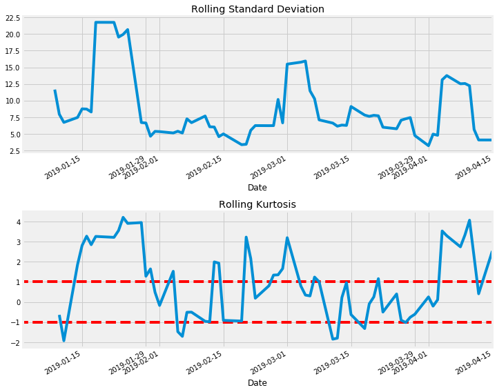
    def plot_rolling_returns(self, show_kurtosis=False):
        """ Convenience function to plot the rolling daily returns (with the specified window, default of 3)
        If show_kurtosis is True, we also plot the rolling Kurtosis values for the specified window. If our returns are truly stationary and therefore follow a normal distribution then this value gives us an indication of how extreme the returns for the previous window (3) days are.    
        """
        assert self.horizon is not None,"Horizon not specified."
        assert self.window is not None,"Window not specified."
        plt.figure(1, figsize=(10,8))
        plt.subplot(211)
        self.data['returns'][:-self.horizon].rolling(self.window).std().plot()
        plt.title('Rolling Standard Deviation')

        plt.subplot(212)
        plt.title('Rolling Kurtosis')
        self.data['returns'][:-self.horizon].rolling(self.window+1).kurt().plot()
        end_date = self.end_date - dt.timedelta(days=self.horizon)
        plt.hlines(y=1, xmin=self.start_date, xmax=end_date, color='r', linestyle='--')
        plt.hlines(y=-1, xmin=self.start_date, xmax=end_date, color='r', linestyle='--')
        plt.tight_layout()
        plt.show()
        
    def print_kurtosis_stats(self):
        assert self.horizon is not None,"Horizon not specified."
        assert self.window is not None,"Window not specified."
        rk = self.data['returns'][:-self.horizon].rolling(self.window).kurt()
        print("Summary Statistics\n", rk.describe())
        # percentage within 1 standard deviation
        print("Percentage of returns within 1 standard deviation: "+"{:.2%}".format(rk.between(-1,1).sum() / rk.shape[0]))
        # percentage within 2 standard deviations
        print("Percentage of returns within 2 standard deviations: "+"{:.2%}".format(rk.between(-2,2).sum() / rk.shape[0]))
        
    def compute_sharp_ratio(self):
        ret = self.data['returns'][1:-horizon].values
        prev = self.data['Adj Close'][:-(horizon+1)].values
        rx = ret/prev
        rf = 0.02141 # for the risk free rate we use the current value (yield) of a 3 month Treasury Bill
        sharp = np.sqrt(252)*np.mean((rx-rf))/np.std(ret)
        return sharp

Tesla

Now we can easily download historical stock data and perform a few statistical tests on it. One of which is Kurtosis, which gives us an indication of where our previous n returns fall on a normal distribution.

tesla = Stock('tsla', start_date, end_date, download_data=True, horizon=10, window=5)
tesla.calculate_returns()
tesla.plot_rolling_returns(show_kurtosis=True)
tesla.print_kurtosis_stats()

Summary Statistics

count    67.000000
mean      0.912019
std       1.765272
min      -2.885840
25%      -0.333411
50%       0.783648
75%       2.480492
max       4.112976
Name: returns, dtype: float64
Percentage of returns within 1 standard deviation: 34.72%
Percentage of returns within 2 standard deviations: 58.33%

You can find the full code here.