
Introduction
In this analysis, I will be building a forecasting (SARIMA) model to trade stocks, particularly:
- Tesla
- Apple
- Amazon
- General Electric
- Boeing
I will be using data from January 1, 2019 though March 28, 2019 for training, and then evaluate this model on April 2019 data. First lets get the stock data.
First, I create a class to contain our stock data, which contains a few convenience methods that we will use to assess assets:
class Stock:
"""Stock object, contains functionality to download historical data
Args:
ticker (str): The ticker of the company that is publicly traded (eg. MSFT for Microsoft)
start_date (:obj:`datetime.datetime`, optional): The date to begin the flow of historical stock data. If not specified, the start date becomes the date when the given ticker was first traded.
end_date (:obj:`datetime.datetime`, optional): The date to conclude the flow of historical stock data. If not specified, will default to the last day data is available (will typically be yesterday)
download_data (bool): Should we go ahead and download the historical stock data?
horizon (:int, optional): The period in days that we wish to forecast
window (:int, optional): The size of the window which is used in rolling window calculations
"""
def __init__(self, ticker, start_date=None, end_date=None, download_data=True, horizon=None, window=None):
self.ticker = ticker
if start_date is not None:
self.start_date = start_date
if end_date is not None:
self.end_date = end_date
if download_data:
self.get_data()
if horizon is not None:
self.horizon = horizon
if window is not None:
self.window = window
def get_data(self):
""" Downloads the historical stock data from Yahoo! Finance
Returns:
True for success, False otherwise.
"""
try:
df = web.DataReader(self.ticker, 'yahoo', self.start_date, self.end_date)
#df.reset_index(inplace=True)
self.data = df
except:
print("Unable to download stock data")
return False
return True
def calculate_returns(self):
""" Calculate the daily returns (lag difference) and adds them to the data """
self.data['returns'] = np.nan
self.data['returns'][1:] = np.diff(self.data['Adj Close'])
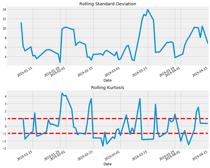
def plot_rolling_returns(self, show_kurtosis=False):
""" Convenience function to plot the rolling daily returns (with the specified window, default of 3)
If show_kurtosis is True, we also plot the rolling Kurtosis values for the specified window. If our returns are truly stationary and therefore follow a normal distribution then this value gives us an indication of how extreme the returns for the previous window (3) days are.
"""
assert self.horizon is not None,"Horizon not specified."
assert self.window is not None,"Window not specified."
plt.figure(1, figsize=(10,8))
plt.subplot(211)
self.data['returns'][:-self.horizon].rolling(self.window).std().plot()
plt.title('Rolling Standard Deviation')
plt.subplot(212)
plt.title('Rolling Kurtosis')
self.data['returns'][:-self.horizon].rolling(self.window+1).kurt().plot()
end_date = self.end_date - dt.timedelta(days=self.horizon)
plt.hlines(y=1, xmin=self.start_date, xmax=end_date, color='r', linestyle='--')
plt.hlines(y=-1, xmin=self.start_date, xmax=end_date, color='r', linestyle='--')
plt.tight_layout()
plt.show()
def print_kurtosis_stats(self):
assert self.horizon is not None,"Horizon not specified."
assert self.window is not None,"Window not specified."
rk = self.data['returns'][:-self.horizon].rolling(self.window).kurt()
print("Summary Statistics\n", rk.describe())
# percentage within 1 standard deviation
print("Percentage of returns within 1 standard deviation: "+"{:.2%}".format(rk.between(-1,1).sum() / rk.shape[0]))
# percentage within 2 standard deviations
print("Percentage of returns within 2 standard deviations: "+"{:.2%}".format(rk.between(-2,2).sum() / rk.shape[0]))
def compute_sharp_ratio(self):
ret = self.data['returns'][1:-horizon].values
prev = self.data['Adj Close'][:-(horizon+1)].values
rx = ret/prev
rf = 0.02141 # for the risk free rate we use the current value (yield) of a 3 month Treasury Bill
sharp = np.sqrt(252)*np.mean((rx-rf))/np.std(ret)
return sharp
Tesla
Now we can easily download historical stock data and perform a few statistical tests on it. One of which is Kurtosis, which gives us an indication of where our previous n returns fall on a normal distribution.
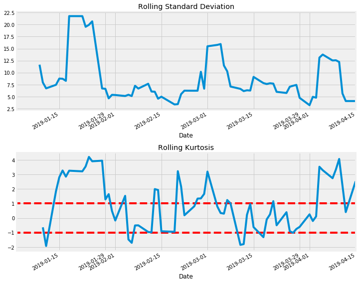
tesla = Stock('tsla', start_date, end_date, download_data=True, horizon=10, window=5)
tesla.calculate_returns()
tesla.plot_rolling_returns(show_kurtosis=True)
tesla.print_kurtosis_stats()
Summary Statistics

count    67.000000
mean      0.912019
std       1.765272
min      -2.885840
25%      -0.333411
50%       0.783648
75%       2.480492
max       4.112976
Name: returns, dtype: float64
Percentage of returns within 1 standard deviation: 34.72%
Percentage of returns within 2 standard deviations: 58.33%
Sharp Ratio: -0.03832159433781627
Apple
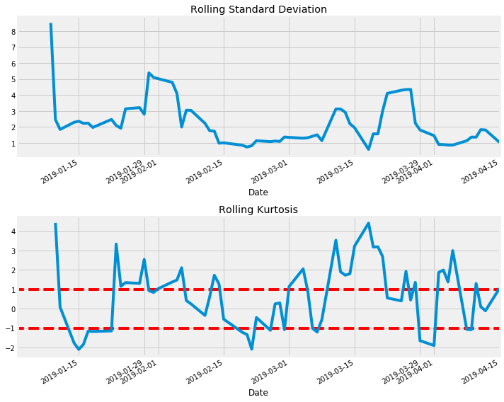
apple = Stock('AAPL', start_date, end_date, download_data=True, horizon=10, window=5)
apple.calculate_returns()
apple.plot_rolling_returns(show_kurtosis=True)
apple.print_kurtosis_stats()
Summary Statistics

count    67.000000
mean      0.664198
std       1.843579
min      -2.846801
25%      -0.860734
50%       0.807611
75%       1.914851
max       4.427327
Name: returns, dtype: float64
Percentage of returns within 1 standard deviation: 31.94%
Percentage of returns within 2 standard deviations: 61.11%
Sharp Ratio: -0.0920835959464692
Amazon
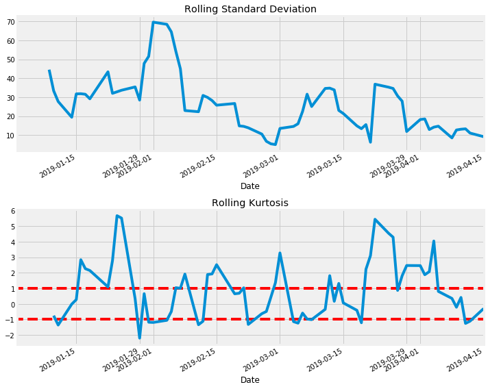
amazon = Stock('AMZN', start_date, end_date, download_data=True, horizon=10, window=5)
amazon.calculate_returns()
amazon.plot_rolling_returns(show_kurtosis=True)
amazon.print_kurtosis_stats()
Summary Statistics

count    67.000000
mean      0.865250
std       2.087454
min      -2.760992
25%      -0.862888
50%       1.096243
75%       2.209349
max       4.863534
Name: returns, dtype: float64
Percentage of returns within 1 standard deviation: 23.61%
Percentage of returns within 2 standard deviations: 59.72%
Sharp Ratio: -0.01020468470365287
General Electric
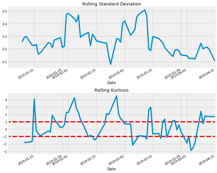
ge = Stock('GE', start_date, end_date, download_data=True, horizon=10, window=5)
ge.calculate_returns()
ge.plot_rolling_returns(show_kurtosis=True)
ge.print_kurtosis_stats()
Summary Statistics

count    67.000000
mean      0.403976
std       1.883122
min      -2.835904
25%      -1.374539
50%       0.737950
75%       1.774063
max       4.250489
Name: returns, dtype: float64
Percentage of returns within 1 standard deviation: 20.83%
Percentage of returns within 2 standard deviations: 59.72%
Sharp Ratio: -1.0768402050313248
Boeing
boeing = Stock('BA', start_date, end_date, download_data=True, horizon=10, window=5)
boeing.calculate_returns()
boeing.plot_rolling_returns(show_kurtosis=True)
boeing.print_kurtosis_stats()
Summary Statistics

count    67.000000
mean     -0.205960
std       2.100253
min      -3.185216
25%      -1.790827
50%      -0.608277
75%       1.548046
max       4.787543
Name: returns, dtype: float64
Percentage of returns within 1 standard deviation: 22.22%
Percentage of returns within 2 standard deviations: 58.33%
Sharp Ratio: -0.03929477241555267
Forecasting: SARIMA
The Seasonal Autoregressive Integrated Moving Average, or SARIMA, model is an approach for modeling univariate time series data that may contain trend and seasonal components. It is an extension on ARIMA models, including new hyperparameters to specify the autoregression (AR), differencing (I), and moving average (MA) for the seasonal component of the series.
Configurations for a SARIMA models include 7 different hyperparameters:
- ARIMA
- p: Trend autoregression order.
- d: Trend difference order.
- q: Trend moving average order
- Seasonal
- P: Seasonal autoregressive order.
- D: Seasonal difference order.
- Q: Seasonal moving average order.
- m: The number of time steps for a single seasonal period.
The trend and seasonal hyperparameters of the model can be configured by analyzing autocorrelation and partial autocorrelation plots, and this can take some expertise. I will use this information, as well as grid searching the hyperparameter space as configurations may not be intuitive. (As this space can get quite large, I will offload this task to more optimized hardware, in this case on Kaggle.) I will use the implementation of SARIMA provided by the statsmodels library.
This model has hyperparameters that control the nature of the model performed for the series, trend and seasonality, specifically:
- order: A tuple p, d, and q parameters for the modeling of the trend.
- sesonal order: A tuple of P, D, Q, and m parameters for the modeling the seasonality
- trend: A parameter for controlling a model of the deterministic trend as one of ‘n’,’c’,’t’,’ct’ for no trend, constant, linear, and constant with linear trend, respectively.
As mentioned above, we can inspect autocorrelation and partial autocorrelation plots in order to determine these parameters, however, I will be developing a grid search framework which will optimize these parameters to minimize error. In this case, I have determined that mean absolute percentage error (MAPE) works better for stock forecasting, as RMSE does not account for the magnitude of assets: 1 share of Google is now at \$1,095.73 and 1 share of Microsoft is at \$134.87, so a 1\% decrease for both would result in a loss of \$10.96 for Google but only a loss of \$1.35 for Microsoft.
Build and Evaluate
I used this script to build and evaluate a SARIMA model, and used this script to grid search the hyperparameter space in order to determine an optimal configuration for the SARIMA model.
Results
Tesla
Tesla’s stock during this period was rather volatile, having a standard deviation of 9.624, a median rolling Kurtosis (window of 5) of 0.784 and a mean of 0.912 and a mean absolute percentage error (MAPE) of 2.165\%. Taking a look at the chart of rolling Kurtosis, it appears to be cyclical: values greater than 0 indicate that that window of returns is on the positive side of the returns distribution (good thing), with this stock spending the majority of time above zero. This information combined with the volatility suggest this is a high risk, high reward stock; depending on your buy/sell signals this asset could be very lucrative but you must have a pretty good appetite for risk.
Now we will forecast 2 business weeks using our SARIMA model:
Recursive Method
# 1 - split the data
train, test = tesla.data[:-horizon]['Adj Close'], tesla.data[-horizon:]['Adj Close']

# 1 - create model
model = SARIMAX(train, order=(1, 1, 1),
                seasonal_order=(0, 0, 0, 0),
                trend='c', enforce_stationarity=False,
                enforce_invertibility=False)

model_fit = model.fit(disp=False)

# recursive method
preds = model_fit.predict(1, len(test))
mean_absolute_percentage_error(test, preds)
Using this method we get a MAPE of 29.51\%, quite poor. If the only deciding factor for keeping or selling a security is the recursive SARIMA model shown above, I would definitely keep TSLA: the last day of my training set has a price of \$267.70 and my model predicts it will close at \$313.88 (an increase of 17.2\%). In fact, my model predicts the price of TSLA will not decrease under the initial amount for the entire horizon of 10 days. However, in actuality if I were to follow this simple model I would lose 9.79\%. On average Tesla stock changes by 2.2%, but our recursive model had a MAPE of over 25%. This is not acceptable, but one of the most basic time series forecasting where the errors are cumulative and explod quickly so not suggested for multi-step forecasting (even with a relatively small horizon).
Let’s improve on this! For this we use the SARIMA Build and Evaluate script mentioned above.
Direct Method
cfg = [(1, 0, 4), (4, 1, 0, 1), 'c']

preds_direct, result = score_model(tesla.data['Adj Close'].values, horizon, cfg)
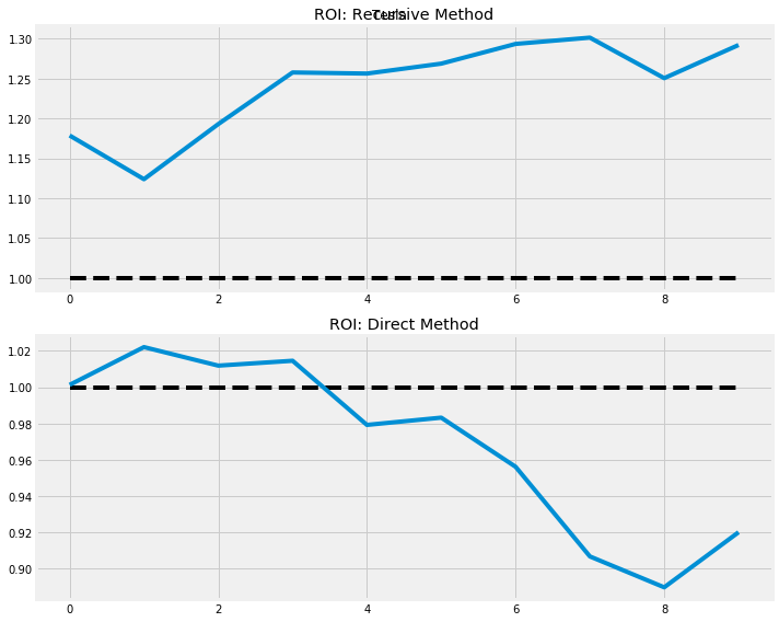
Tihs model achieves a MAPE of 1.955\%, much better! This model essentially predicts the opposite of the recursive SARIMA model: of the 10 day horizon only 3 days are predicted to be be gains versus all 10 for the recursive model. This model predicts a slight decrease in closing price for the first day of our horizon, so we should use another metric in combination with this information in deciding to keep or sell this security. In comes the Sharp Ratio, where we use the rate of a 3 month treasury bill in order to calculate excess returns (2.149\% found here).
\[S_r = \frac{\hat{r_p}-r_f}{\sigma}\]To finish this article we need to annualize the Sharpe ratio, since we calculated it from daily values. There are 252 trading days in the year, so the simple way to annualize it is to multiply the Sharpe ratio by the square root of 252. As reported above, Tesla has an annualized Sharp Ratio of -0.0383, so using this value as well as the forecasted prices I would sell this stock (or at the least decrease my position).
Evaluate
y_true = tesla[-(n_test+1):-1]['y'].values
y_pred = np.array(preds[-n_test:])
mean_absolute_percentage_error(y_true, y_pred)
Using the direct strategy for multi-step forecasting reduced our mean absolute percentage error to 1.003! While this is lower than the volatility inherent in the stock data, the rolling Kurtosis values and high volatility would cause me to be skeptical so I would not hold (or even buy in the first place).
Apple
The full source code can be found here.